There are four basic image types: binary, grayscale,
truecolor, and indexed images. Here are some examples of each type together
with their information.
Note: imfinfo outputs the following image information->
File Name, File size (bytes), Width, Height, bit depth, and Color type
1. Binary image

Image taken from:
The extracted image information using Scilab imfinfo are:

(The bit depth is 8 because imfinfo in SVIP module only
outputs either grayscale or true color and represents the 1’s and 0’s of a
binary image with 255 and 0 as shown below.)


Image taken from:
Image information:
3. Truecolor images

Image taken from:
Image information:

*note the addition of another channel in the image array which gives the RGB values of each pixel in the image.
4. Indexed images
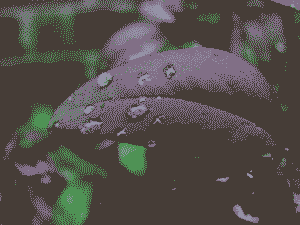
Image taken from:
Image information:

The color map of the image was obtained from Gimp v2.8:

Some of the more advanced image types are as follows:
1. High dynamic range (HDR) images

Image taken from:
2. Multi-/Hyper-spectral images

Image taken from: http://www.fas.org/irp/imint/docs/rst/Intro/Part2_26.html
3.

Image taken from: http://3d-wallpapers.net/3d-pictures
Now, it's time to do some image processing. First, we try to convert a truecolor image to grayscale and binary images using the rgbtogray and im2bw commands. In this example we will use the following 1280pixels x 800pixels true color image with array size of 800x1280x3:

Image taken from: //www.wuala.com/nknwn666/random%20wallpapers,%20pics%20
(mostly%20anime)/anime_wallpapers_mOole.ru_122.jpg/
Converted to grayscale, the image now only has a single
layer making its array size just 800x1280.

When converted to binary form using a threshold value of
0.5, that is, a pixel which has a value greater than 255*0.5 will be assigned a
value of 1 and 0, otherwise. Note that its array size is similar to that of
a grayscale image.

The code used to do these is as follows:
stacksize(100000000);//set stacksize
I = imread('C:\Users\Tin\Desktop\AP_186\Act3\anime.jpg');
conv = rgb2gray(I);//convert to grayscale
imwrite(conv, "grayscaled.png")//save grayscaled image
BW = im2bw(conv,0.6)//convert to bw image
imwrite(BW,"thr_0.6.png");//save bw image


Taking the histogram of the image, I got:

From the histogram, I selected
the threshold to be at 150, which is approximately the point where the
distribution starts to flatten. The pixels with values greater than 150 may already
be contributions from the lighter background, especially those which result
from scanning the page. The threshold value used for the imhist command is then 150/255 ~ 0.6 The resulting binary image is shown below.

The implemented threshold has
effectively separated the lines in the graph from the background. I tried to
use other threshold values that are higher and lower than 0.6. When the
threshold is decreased, the lines become fainter, and when it is increased they
become darker and the dark areas due to the scan become visible. The results are shown below (left: threshold = 0.5; right: threshold = 0.7):


The code used for this part is as follows:
stacksize(100000000);//set stacksize
In this activity, I saved all the images that I produced in PNG format. There are other formats in which images may be saved depending on the required image size and quality. The following are some of them:
stacksize(100000000);//set stacksize
I = imread('C:\Users\Tin\Desktop\AP_186\Act3\scan0033_2.jpg');
conv = rgb2gray(I);//convert to grayscale
imwrite(conv, "grayscaled.png")//save grayscaled image
[counts, cells]=imhist(conv);//take histogram of grayscaled image
histplot(cells, counts);//plot histogram
BW = im2bw(conv,0.6)//convert to bw image
imwrite(BW,"thr_0.6.png");//save bw image
In this activity, I saved all the images that I produced in PNG format. There are other formats in which images may be saved depending on the required image size and quality. The following are some of them:
- JPEG format - The Joint Photographic Experts Group has developed the JPEG file format. It is good for use in photographic images. Most images captured by cameras, are saved in JPEG format because of its compact size which makes it easier for processing. However, this portability comes at the expense of lossy image compression which reduces the quality of the saved image.
- BMP or Bitmap image file, also known as device-independent bitmap, is the standard format for Windows operating system which stores bitmap images. It supports 2D images with various dimensions, resolutions, color type, and color depth. It is impractical to use on the web because of the large file size of images in this format.
- GIF or Graphic Interchange format is an image file format developed by Compuserve which allows animations but is limited when it comes to color representations. It can only support up to 256 colors, unlike its counterparts. Hence, it is not ideal for use in application such as photography and archiving.
- PNG, which stands for Portable Network Graphic, is a lossless image compression format which was developed mainly to overcome the limitations of the GIF format. It employs a compression technique called deflation. It allows storage of more image attributes and larger greater bit depths. In particular, PNG files may store gamma values, background color, and textual information. The standard allows up to 16 bits for each color channel. PNG files may be used in many different application and is supported by the web.
- TIFF or Tagged Image File Format is another lossless image compression format developed by Aldus (now Adobe Systems) which delivers high quality images but at the cost of larger file sizes. Basic TIFF images include bilevel, grayscale, palette/indexed, and true color (RGB). RGB TIFF images are capable of holding up to 16.7M colors while indexed and grayscale images only have 256 colors or shades. TIFF images are mostly used for archiving important images. Due to its large file size, there is little support for TIFF images on the web.
References:
1. http://www.coolutils.com/bmp
2. http://www.coolutils.com/gif
3. http://www.coolutils.com/jpeg
4. http://www.fileformat.info/format/png/corion.htm
5. http://kb.iu.edu/data/afjn.html
Comments
Post a Comment