IN this activity, we will try to
enhance an image by manipulating its histogram. By enhance, I mean the improvement of a dark image such that features disguised by the dark areas may be revealed. The histogram of a graylevel
image, when normalized to the number of pixels, gives us the probability
distribution function (PDF).
For example, if we have the following color
image:
Then, convert it to a graylevel image using Scilab:
 |
| Figure 1b. Grayscaled version of the image in Figure 1a |
We get its PDF by dividing
each pixel by the total number of pixels.
 |
| Figure 1c. Code for obtaining PDF of image |
 |
| Figure 1d. PDF of the graylevel image |
From the PDF, we see that the distribution is biased towards the low values.
If the image has graylevels, r,
with a PDF of p1(r) and a cumulative distribution function (CDF) given by,
then we can map it to a new set of graylevels, z, described
by a different CDF described by:
where p2(z) is the new PDF of the image.
This technique is called backprojection and is best illustrated by the diagram
found in Figure 2.
 |
| Figure 2. Illustration of the backprojection method. Look for the graylevel value, r, of the pixel, and find its corresponding CDF value T(r). Project the value of T(r) for the graylevel on the desired CDF , G(z). Look for the graylevel value which corresponds to the mapped value for G(z). This graylevel value will replace the original value. |
For the image in Figure 1b, we
determine the CDF using the cumsum() command in SciLab as shown in the code
snippet in Figure 3. The CDF is shown in Figure 4.
 |
| Figure 3. Code for obtaining CDF of image |
 |
| Figure 4. CDF of the graylevel image in Figure 1b. |
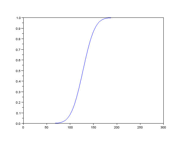
We then map the y values from the
original CDF to a desired CDF. In this case we used a linear CDF and the CDF of
a Gaussian PDF as shown in Figure 5.
 |
| Figure 5a. Linear CDF |
 |
| Figure 5b. CDF of Gaussian PDF |
We then use the interp() function
in SciLab to find the corresponding graylevel value, z, for the y value that we
mapped on the desired CDF. We then replace the graylevel value for each pixel
of the original image by the new grayvalue obtained from the backprojection
method. The code used to do this is shown below.
Shown below are the enhanced images
using the linear CDF and the CDF of a Gaussian PDF. The corresponding CDFs of the enhanced images are also shown.
 |
| Figure 6a. Image enhanced using a linear CDF |
 |
| Figure 6b. CDF of the image in Figure 6a. |
 |
| Figure 6c. Enhanced image using CDF for a Gaussian PDF |
 |
| Figure 6d. CDF of image in Figure 6c |
The enhanced images show some feature that we cannot see just by looking at the original grayscale image such as some of the features of the branches and leaves of the surrounding trees. The image which resulted from the projection on a linear CDF is sharper compared to that obtained for the CDF of a Gaussian PDF. However, the image is too bright making some parts of the image to be indistinguishable due to the brightness. For the enhanced image using the CDF of a Gaussian PDF, the contrast is not as sharp and most parts of the original image are still distinguishable.
For this activity, I would like to thank Ms. Eloisa Ventura, Ms. Maria Isabel Saludares and Mr. Benjur Borja for useful discussions.
Finally, I give myself a grade of 10/10 for being able to fulfill the requirements in the activity.
References:
1. M. Soriano, A5: Enhancement by Histogram Manipulation Manual, 2012
 then we can map it to a new set of graylevels, z, described
by a different CDF described by:
then we can map it to a new set of graylevels, z, described
by a different CDF described by: where p2(z) is the new PDF of the image.
This technique is called backprojection and is best illustrated by the diagram
found in Figure 2.
where p2(z) is the new PDF of the image.
This technique is called backprojection and is best illustrated by the diagram
found in Figure 2.




Comments
Post a Comment