Activity 2: SciLab basics

For the second activity we had a bit of practice in using the SciLab programming language. We had to produce the following synthetic images:

1. a.       Centered square aperture
2. b.      Sine wave along x direction (corrugated roof)
3. c.       Grating along x direction
4. d.      Annulus
5. e.      Circular aperture with graded transparency (Gaussian function)

But first we had to follow a sample code given by Dr. Soriano. The code produced a 100 x 100 pixel – image of a centered circular aperture with radius of 35 pixels (Figure 1).

Figure 1. Code and synthetic image for centered circular aperture

After doing the centered circular aperture I am ready to do the other synthetic images.

The easiest was the annulus since you just have to tweak the code for the centered circular aperture. I just replaced line 7 of the code with: A(find(r<0.7 & r>0.3)) = 1. This logical statement would only return True for regions between circles with r<0.7 and r>0.3, hence, only this interval would have a value 1 giving us an annulus (Figure 2). To change the thickness of the annulus, you just have to change the values for the radii.

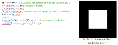
 I used 500 x 500 pixels for my image dimensions for this and all the other images.

Figure 2. Code and synthetic image for annulus

The centered square aperture was fairly easy to do. It’s still similar to that of the centered aperture but this time you have to find values of x and y that are less than a certain value s which corresponds to the length of a side. The code and the resulting image is shown in Figure 3.

Figure 3. Code and synthetic image for centered square aperture

Next is the corrugated roof done using a sine function along the x-direction. The code and results are found in Figure 4. 

Figure 4. Code and synthetic image for sinusoid along x direction 

To create the grating, I used a sinusoid along the x direction. I just replaced the values in the matrix that are greater than 0 with 1, and those less than or equal to 0 with 0. The code and results are shown below (Figure 5). 

Figure 5. Code and synthetic image for grating along x direction 

Finally, for the circular aperture with graded transparency, I just multiplied the aperture matrix with the Gaussian mask matrix which I produced by using the Gaussian function. For different values of the parameter c,which gives the variance of the Gaussian function, the resulting image also varies. Code and image found in Figure 6.

Figure 6. Code and synthetic image for circular aperture 

with graded transparency (Gaussian function)

Here are some other images that I tried, the criss-cross pattern and the double slit:

Code Snippet:

//cross

x2 = linspace(-7*%pi, 8*%pi, 500)

y2 = sin(x2);

grating = ndgrid(y2,y2);

grating(find(grating>0))= 0;

grating(find(grating<=0))= 1;

checkerboard = grating'- grating;

imwrite(checkerboard, "cross.png");

//double slit

nx = 200;

grid = zeros(nx, nx)

dist = 20;

width = 30;

ind1 = nx/2 -dist/2;

ind2 = nx/2 +dist/2;

grid(1:nx,ind1-width:ind1) = 1;

grid(1:nx,ind2:ind2+width) = 1;

imwrite(grid, "double_slit.png");

For this activity, I give myself a grade of 12/10 because I was able to produce all the required synthetic images and took the initiative to create other patterns. I also think that the codes that I used were efficient and effective. :D

I would like to thank Ms. Mabel Saludares and Mr. Gino Borja for helpful discussions. :)